コマンドラインから高度なプロット

この投稿は、MATLABからカスタムプロットを受け付けています。 EEGLABメニュー

トピックス

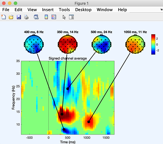
すべての電極上の時間周波数プロット

この例では、低レベルの電力の一部を示しています現在利用可能な機能の範囲を超えて行くスクリプトグラフィカル以下は、このスクリプトをチュートリアルのepochedデータセットで実行します。参照: tftopo.mの関数は強力な機能ですすべてのチャネルで時間の頻度分解をプロットできます。

% Compute a time-frequency decomposition for every electrode
eeglab; close; % add path
eeglabp = fileparts(which('eeglab.m'));
EEG = pop_loadset(fullfile(eeglabp, 'sample_data', 'eeglab_data_epochs_ica.set'));
for elec = 1:EEG.nbchan
    [ersp,itc,powbase,times,freqs,erspboot,itcboot] = pop_newtimef(EEG, …
    1, elec, [EEG.xmin EEG.xmax]*1000, [3 0.5], 'maxfreq', 50, 'padratio', 16, ...
    'plotphase', 'off', 'timesout', 60, 'alpha', .05, 'plotersp','off', 'plotitc','off');
    if elec == 1  % create empty arrays if first electrode
        allersp = zeros([ size(ersp) EEG.nbchan]);
        allitc = zeros([ size(itc) EEG.nbchan]);
        allpowbase = zeros([ size(powbase) EEG.nbchan]);
        alltimes = zeros([ size(times) EEG.nbchan]);
        allfreqs = zeros([ size(freqs) EEG.nbchan]);
        allerspboot = zeros([ size(erspboot) EEG.nbchan]);
        allitcboot = zeros([ size(itcboot) EEG.nbchan]);
    end;
    allersp (:,:,elec) = ersp;
    allitc (:,:,elec) = itc;
    allpowbase (:,:,elec) = powbase;
    alltimes (:,:,elec) = times;
    allfreqs (:,:,elec) = freqs;
    allerspboot (:,:,elec) = erspboot;
    allitcboot (:,:,elec) = itcboot;
end;
% Plot a tftopo() figure summarizing all the time/frequency transforms
figure;
tftopo(allersp,alltimes(:,:,1),allfreqs(:,:,1),'mode','ave','limits', …
[nan nan nan 35 -1.5 1.5],'signifs', allerspboot, 'sigthresh', [6], 'timefreqs', ...
[400 8; 350 14; 500 24; 1050 11], 'chanlocs', EEG.chanlocs);

スクリプトは、次の図を生成します。

この関数は、CenterP の出力を、バイナリ統計解析で行います。

スカルプトポグラフィにおけるプロット対策

プロットの時間頻度分解

参照: 特注品関数は強力な機能ですすべてのチャネルおよびコンポーネントのあらゆる測定をプロットできます。例えば、下のコードは時間頻度の分解をのためのプロットすることを可能にしますすべてのデータチャネル。

eeglab; close; % add path
eeglabp = fileparts(which('eeglab.m'));
EEG = pop_loadset(fullfile(eeglabp, 'sample_data', 'eeglab_data_epochs_ica.set'));
figure; metaplottopo( EEG.data, 'plotfunc', 'newtimef', 'chanlocs', EEG.chanlocs, 'plotargs', ...
                   {EEG.pnts, [EEG.xmin EEG.xmax]*1000, EEG.srate, [0], 'plotitc', 'off', 'ntimesout', 50, 'padratio', 1});

PlotのERP

次の例では、すべてのデータをERPimage にプロットする。 ERPimage では、各関数の軸線が点在しています。必要に応じて、何百ものチャンネルをプロットするのが便利です。 ICA交換する EEGデータと EEG.icaact と ‘chanlocs’ は、外に渡します。

figure; metaplottopo( EEG.data, 'plotfunc', 'erpimage', 'chanlocs', EEG.chanlocs, 'plotargs', ...
         { eeg_getepochevent( EEG, {'rt'},[],'latency') linspace(EEG.xmin*1000, EEG.xmax*1000, EEG.pnts) '' 10 0 });

スカルプトポグラフィアニメーション制作

このページで使用されるスクリプトは、 m 点

eegmovie関数2Dspcaltopoグラフィアニメーション

scalpMap アニメーションへスキップ(limited) eegmovie。 m 点コマンドラインから。例えば、レイテンシー範囲のムービーを作るために-100ミリ秒から600ミリ秒、タイプ:

%% Simple 2-D movie
eeglab; close; % add path
eeglabp = fileparts(which('eeglab.m'));
EEG = pop_loadset(fullfile(eeglabp, 'sample_data', 'eeglab_data_epochs_ica.set'));

% Above, convert latencies in ms to data point indices
pnts1 = round(eeg_lat2point(-100/1000, 1, EEG.srate, [EEG.xmin EEG.xmax]));
pnts2 = round(eeg_lat2point( 600/1000, 1, EEG.srate, [EEG.xmin EEG.xmax]));
scalpERP = mean(EEG.data(:,pnts1:pnts2),3);

% Smooth data
for iChan = 1:size(scalpERP,1)
    scalpERP(iChan,:) = conv(scalpERP(iChan,:) ,ones(1,5)/5, 'same');
end

% 2-D movie
figure; [Movie,Colormap] = eegmovie(scalpERP, EEG.srate, EEG.chanlocs, 'framenum', 'off', 'vert', 0, 'startsec', -0.1, 'topoplotopt', {'numcontour' 0});
seemovie(Movie,-5,Colormap);

% save movie
vidObj = VideoWriter('erpmovie2d.mp4', 'MPEG-4');
open(vidObj);
writeVideo(vidObj, Movie);
close(vidObj);

3DヘッドプロットでERPをプロットする機能

eegmovie関数3Dsプカルトポグラフィ

下の下のはははははは

%% Simple 3-D movie
% Use the graphic interface to coregister your head model with your electrode positions
headplotparams1 = { 'meshfile', 'mheadnew.mat'       , 'transform', [0.664455     -3.39403     -14.2521  -0.00241453     0.015519     -1.55584           11      10.1455           12] };
headplotparams2 = { 'meshfile', 'colin27headmesh.mat', 'transform', [0          -13            0          0.1            0        -1.57         11.7         12.5           12] };
headplotparams  = headplotparams1; % switch here between 1 and 2

% set up the spline file
headplot('setup', EEG.chanlocs, 'STUDY_headplot.spl', headplotparams{:}); close
 
% check scalp topo and head topo
figure; headplot(scalpERP(:,end-50), 'STUDY_headplot.spl', headplotparams{:}, 'maplimits', 'absmax', 'lighting', 'on');
figure; topoplot(scalpERP(:,end-50), EEG.chanlocs);
figure('color', 'w'); [Movie,Colormap] = eegmovie( scalpERP, EEG.srate, EEG.chanlocs, 'framenum', 'off', 'vert', 0, 'startsec', -0.1, 'mode', '3d', 'headplotopt', { headplotparams{:}, 'material', 'metal'}, 'camerapath', [-127 2 30 0]); 
seemovie(Movie,-5,Colormap);

% save movie
vidObj = VideoWriter('erpmovie3d1.mp4', 'MPEG-4');
open(vidObj);
writeVideo(vidObj, Movie);
close(vidObj);

「ヘッドプラム = headplotparams1;」を「headplotparams = headplotparams2;」に改行して、ヘッドモデルをモデル化します。

次のセクションに示すように映画用のフレームを作成することもできます。

フレームから映画を作る

別のソリューションは、映画に一連の画像を組み立てることです。例:

%% Using topoplot to make movie frames
vidObj = VideoWriter('erpmovietopoplot.mp4', 'MPEG-4');
open(vidObj);
counter = 0;
for latency = -100:10:600 %-100 ms to 1000 ms with 10 time steps
    figure; pop_topoplot(EEG,1,latency, 'My movie', [] ,'electrodes', 'off'); % plot'
    currFrame = getframe(gcf);
    writeVideo(vidObj,currFrame);
    close;  % close current figure
end
close(vidObj);