統計コースプロット
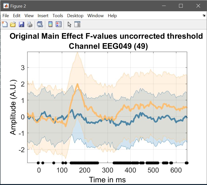
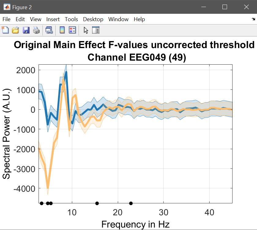
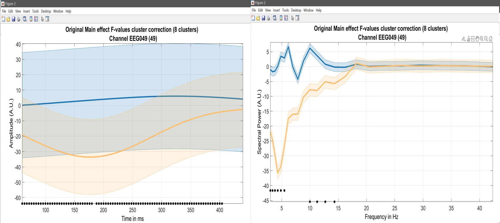
統計的な結果が出た場合、’image all’ は、すべての F と p-values とクラスター (計算された場合) 、’course plot’ も指定されたチャネルに対する効果の時間経過を示しています。 ANOVAは1ウェイで、Fテストは2つの同時コントラスト(A>BとB>Cを知っている場合、A>Cと実際の統計テストはすべての違いを計算する必要はありません)のみを伴うため、通常は3つの条件の2つの曲線になります。 対照的に、これは唯一の1曲線であり、(トリミング)が0に等しい差を意味した場合のテスト(例えば。 図 17).
ここでは、片道のANOVAを計算した後、このケースは、タイプです。 load('LIMO.mat'); LIMO.design.C{1} そして、結果は、馴染みのあると非familiarの顔とスクランブルと非familiarの顔の間([1 0 -1; 0 1 -1])の間の平均差のためにテストされた行列で、2曲線をプロットする - (図 23 のために ERP, スペクトル そして、 ERSP).
limo_display_results(3,'Rep_ANOVA_Main_effect_1_face.mat',pwd,0.05,2,...
    fullfile(pwd,'LIMO.mat'),0,'channels',49,'sumstats','mean'); % course plot
saveas(gcf, 'Rep_ANOVA_Main_effect_timecourse.fig'); close(gcf)
limo_display_results(3,'Rep_ANOVA_Main_effect_1_face.mat',pwd,0.05,2,...
    fullfile(pwd,'LIMO.mat'),0,'channels',49,'sumstats','mean'); % spectrum plot
saveas(gcf, 'Rep_ANOVA_Main_effect_spectrum.fig'); close(gcf)
limo_display_results(3,'Rep_ANOVA_Main_effect_1_face.mat',pwd,0.05,2,...
    fullfile(pwd,'LIMO.mat'),0,'channels',49,'restrict','time','dimvalue',5,'sumstats','mean'); % course plot
saveas(gcf, 'Rep_ANOVA_Main_effect_5Hztimecourse.fig'); close(gcf)
limo_display_results(3,'Rep_ANOVA_Main_effect_1_face.mat',pwd,0.05,2,...
    fullfile(pwd,'LIMO.mat'),0,'channels',49,'restrict','frequency','dimvalue',180,'sumstats','mean'); % course plot
saveas(gcf, 'Rep_ANOVA_Main_effect_180msSpectrum.fig'); close(gcf)
Figure 23. ANOVAのコースプロット
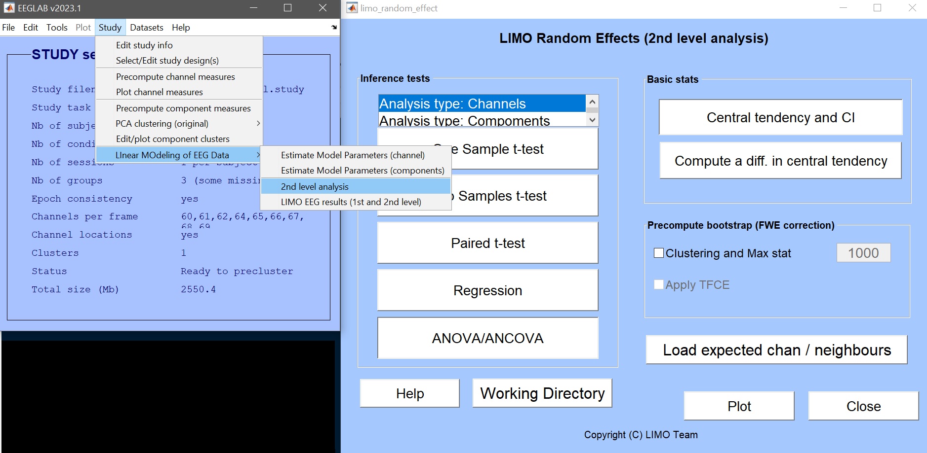
しかし、データへの結果を関連付けることも重要です。 そのためには、平均値を計算し、効果サイズをチェックすることができます。 2ndレベルメニューから実現できます。図9)「基本統計」サブメニューを通して。
統計効果のサイズ
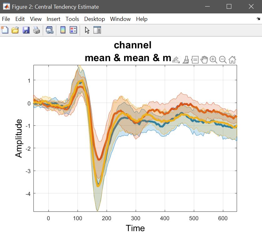
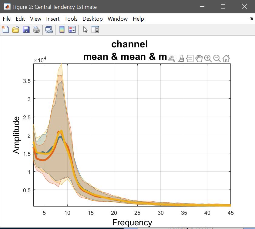
ANOVAは、ベータパラメータ、またはリニアコンビネーションで計算されています。 LIMOを使用して自信の間隔を持つ手段は、Centralの傾向とCIを選ぶことができます。 繰り返された対策 ANOVA は、means で計算されています。ここでは、それぞれのコントラスト(つまり、con1 のリストを選択し、con2 と con3 を繰り返します)の意味を計算します。図 24)。 *plot 中央傾向と差** を使用して結果を視覚化 - 図 25 のために ERP, スペクトル そして、 ERSP.
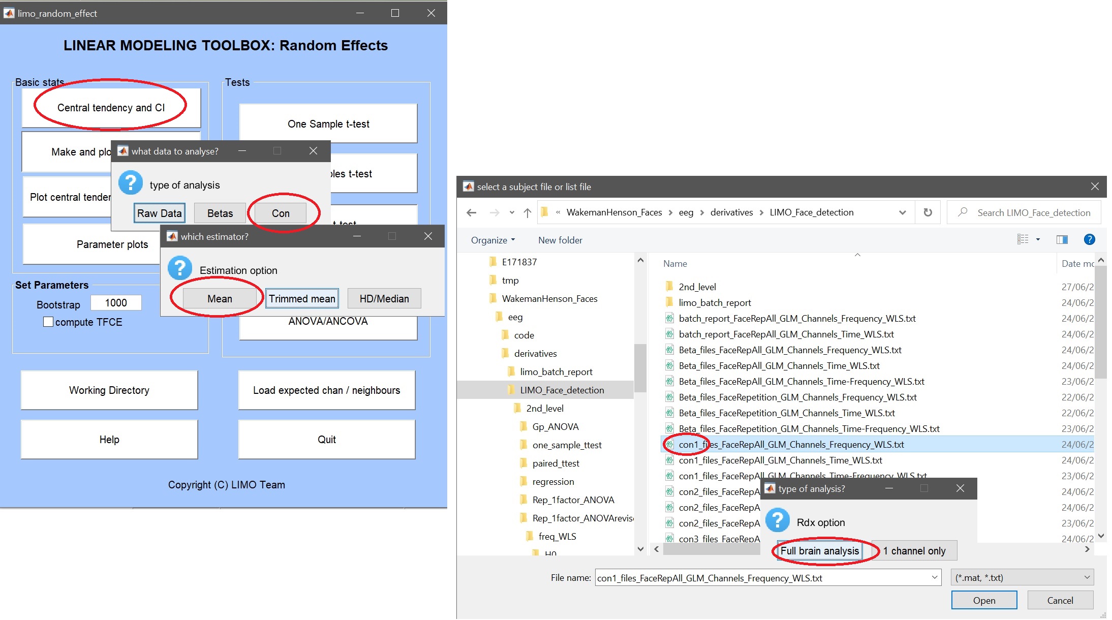 Figure 24. 中央傾向と CI の GUI, データの種類 (例: con), 要約統計 (例: 平均), ファイルまたはリスト (.txt) ファイルとチャンネル (例: 完全な脳).
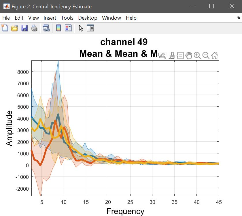
Yr       = load('Yr.mat'); % ANOVA data are channel*[freq/time]frames*subjects*conditions
chanlocs = [STUDY.filepath filesep 'limo_gp_level_chanlocs.mat'];
mkdir('average_betas'); cd('average_betas');
limo_central_tendency_and_ci(squeeze(Yr.Yr(:,:,:,1)), 'Mean',[],fullfile(pwd,'famous.mat'))
limo_central_tendency_and_ci(squeeze(Yr.Yr(:,:,:,2)), 'Mean',[],fullfile(pwd,'scrambled.mat'))
limo_central_tendency_and_ci(squeeze(Yr.Yr(:,:,:,3)), 'Mean',[],fullfile(pwd,'unfamiliar.mat'))
limo_add_plots('channel',49,fullfile(fileparts(pwd),'LIMO.mat'),...
    {fullfile(pwd,'famous_Mean.mat'), fullfile(pwd,'scrambled_Mean.mat'), fullfile(pwd,'unfamiliar_Mean.mat')})
title('mean betas channel 49'); saveas(gcf, 'Rep_ANOVA_Main_effect_Betas.fig'); close(gcf)
Yr       = load('Yr.mat'); % ANOVA data are channel*[freq/time]frames*subjects*conditions
chanlocs = [STUDY.filepath filesep 'limo_gp_level_chanlocs.mat'];
mkdir('average_betas'); cd('average_betas');
limo_central_tendency_and_ci(squeeze(Yr.Yr(:,:,:,:,1)), 'Mean',[],fullfile(pwd,'famous.mat'))
limo_central_tendency_and_ci(squeeze(Yr.Yr(:,:,:,:,2)), 'Mean',[],fullfile(pwd,'scrambled.mat'))
limo_central_tendency_and_ci(squeeze(Yr.Yr(:,:,:,:,3)), 'Mean',[],fullfile(pwd,'unfamiliar.mat'))
limo_add_plots('channel',49,'restrict','time','dimvalue',5,fullfile(fileparts(pwd),'LIMO.mat'),...
    {fullfile(pwd,'famous_Mean.mat'), fullfile(pwd,'scrambled_Mean.mat'), fullfile(pwd,'unfamiliar_Mean.mat')})
title('mean betas channel 49 @5Hz'); saveas(gcf, 'Rep_ANOVA_Main_effect_Betas5Hz.fig'); close(gcf)
limo_add_plots('channel',49,'restrict','frequency','dimvalue',180,fullfile(fileparts(pwd),'LIMO.mat'),...
    {fullfile(pwd,'famous_Mean.mat'), fullfile(pwd,'scrambled_Mean.mat'), fullfile(pwd,'unfamiliar_Mean.mat')})
title('mean betas channel 49 @180ms'); saveas(gcf, 'Rep_ANOVA_Main_effect_Betas180ms.fig'); close(gcf)
図25. 平均値.
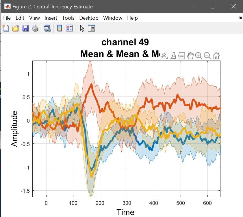
未加工データ効果のサイズ
計算中、ベータ/コンの手段またはトリムされた手段 (1) は 2 番目のレベルで行われる計算を反映し、(2) は結果を理解することができます。結果を解釈するために必要な基礎的なデータと未加工効果のサイズを示すものではありません。 これは、中央傾向とCIを「Raw Data」で計算したいことを意味します。 図 26)。 LIMOファイルのリストを選択し、有名な顔の[1 2 3]、スクランブルされた顔の[4 5 6]、および[7 8 9]を選択します。 あなたは興味のチャネルや脳の分析のためにそれを行うオプションを持っています, そして、あなたの推定者を使用します. ここでは、各試験からの重量を使用して、各条件のマイアンを見たいです(WLSを使用した第1レベル)。 あらゆる条件で繰り返す必要があります。 2番目のレベルのメニューまたは結果メニューの「プロット中央傾向と違い」を使用して、それらの平均をプロットすることができます。 結果は図27で示されています ERP, スペクトラム そして、 ERSP.
LIMOfiles = fullfile(STUDY.filepath,['LIMO_' STUDY.filename(1:end-6)],'LIMO_files_FaceRepAll_GLM_Channels_Time_WLS.txt');
mkdir('ERPs'); cd('ERPs');
limo_central_tendency_and_ci(LIMOfiles, [1 2 3], chanlocs, 'Weighted mean', 'Mean', [],fullfile(pwd,'famous.mat'))
limo_central_tendency_and_ci(LIMOfiles, [4 5 6], chanlocs, 'Weighted mean', 'Mean', [],fullfile(pwd,'scrambled.mat'))
limo_central_tendency_and_ci(LIMOfiles, [7 8 9], chanlocs, 'Weighted mean', 'Mean', [],fullfile(pwd,'unfamiliar.mat'))
limo_add_plots('channel',49,fullfile(fileparts(pwd),'LIMO.mat'),...
    {fullfile(pwd,'famous_Mean_of_Weighted mean.mat'),fullfile(pwd,'scrambled_Mean_of_Weighted mean.mat'),...
    fullfile(pwd,'unfamiliar_Mean_of_Weighted mean.mat')}); title('ERPs channel 49')
saveas(gcf, 'Rep_ANOVA_Main_effectERP.fig'); close(gcf)
LIMOfiles = fullfile(STUDY.filepath,['LIMO_' STUDY.filename(1:end-6)],'LIMO_files_FaceRepAll_GLM_Channels_Frequency_WLS.txt');
mkdir('ERPs'); cd('ERPs');
limo_central_tendency_and_ci(LIMOfiles, [1 2 3], chanlocs, 'Weighted mean', 'Mean', [],fullfile(pwd,'famous.mat'))
limo_central_tendency_and_ci(LIMOfiles, [4 5 6], chanlocs, 'Weighted mean', 'Mean', [],fullfile(pwd,'scrambled.mat'))
limo_central_tendency_and_ci(LIMOfiles, [7 8 9], chanlocs, 'Weighted mean', 'Mean', [],fullfile(pwd,'unfamiliar.mat'))
limo_add_plots('channel',49,fullfile(fileparts(pwd),'LIMO.mat'),...
    {fullfile(pwd,'famous_Mean_of_Weighted mean.mat'),fullfile(pwd,'scrambled_Mean_of_Weighted mean.mat'),...
    fullfile(pwd,'unfamiliar_Mean_of_Weighted mean.mat')}); title('ERPs channel 49')
saveas(gcf, 'Rep_ANOVA_Main_effectSpectrum.fig'); close(gcf)
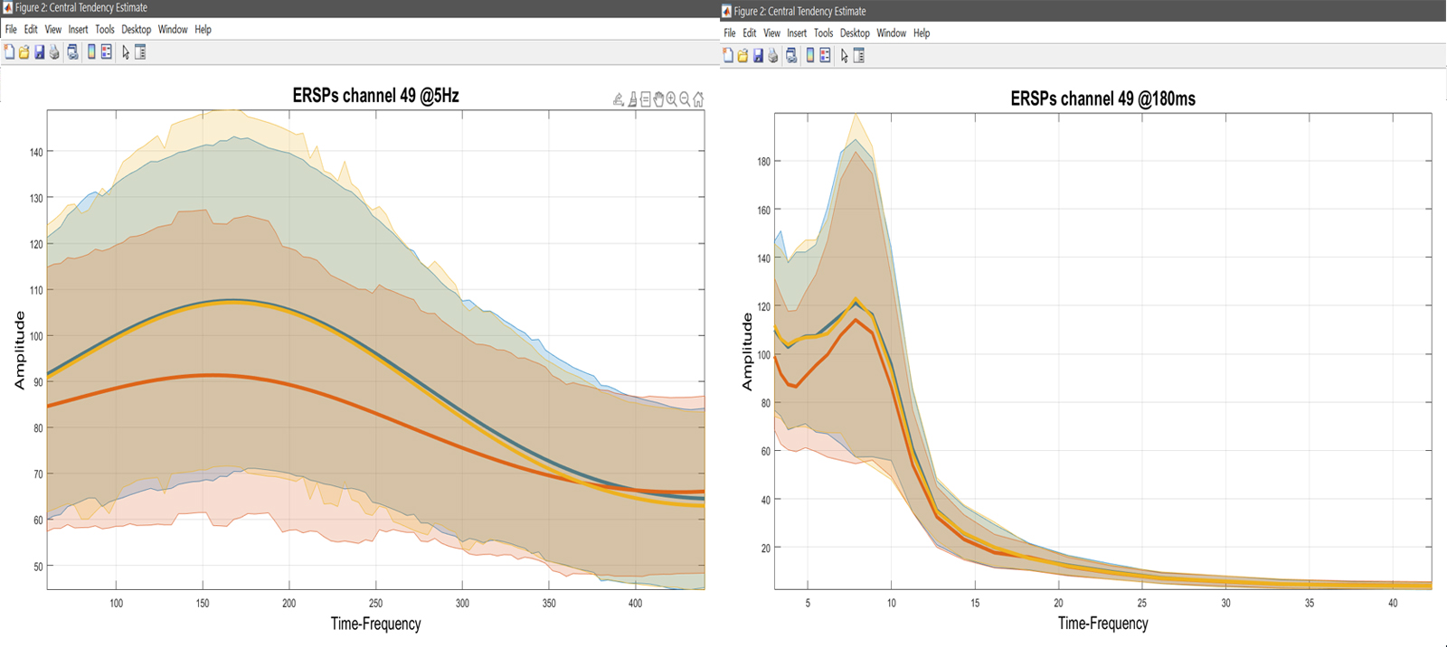
LIMOfiles = fullfile(STUDY.filepath,['LIMO_' STUDY.filename(1:end-6)],'LIMO_files_FaceRepAll_GLM_Channels_Time-Frequency_WLS.txt');
mkdir('ERSPs'); cd('ERSPs');
limo_central_tendency_and_ci(LIMOfiles, [1 2 3], chanlocs, 'Weighted mean', 'Mean', [],fullfile(pwd,'famous.mat'))
limo_central_tendency_and_ci(LIMOfiles, [4 5 6], chanlocs, 'Weighted mean', 'Mean', [],fullfile(pwd,'scrambled.mat'))
limo_central_tendency_and_ci(LIMOfiles, [7 8 9], chanlocs, 'Weighted mean', 'Mean', [],fullfile(pwd,'unfamiliar.mat'))
limo_add_plots('channel',49,'restrict','Time','dimvalue',5,fullfile(fileparts(pwd),'LIMO.mat'),...
    {fullfile(pwd,'famous_Mean_of_Weighted mean.mat'),fullfile(pwd,'scrambled_Mean_of_Weighted mean.mat'),...
    fullfile(pwd,'unfamiliar_Mean_of_Weighted mean.mat')}); title('ERSPs channel 49 @5Hz')
saveas(gcf, 'Rep_ANOVA_Main_effect_ERSPs5Hz.fig'); close(gcf)
limo_add_plots('channel',49,'restrict','Frequency','dimvalue',180,fullfile(fileparts(pwd),'LIMO.mat'),...
    {fullfile(pwd,'famous_Mean_of_Weighted mean.mat'),fullfile(pwd,'scrambled_Mean_of_Weighted mean.mat'),...
    fullfile(pwd,'unfamiliar_Mean_of_Weighted mean.mat')}); title('ERSPs channel 49 @180ms')
saveas(gcf, 'Rep_ANOVA_Main_effect_ERSPs180msz.fig'); close(gcf)
_Figure 27. 被験者全体の平均データ(重み付きトライアルを使用). ツイート
図を作成するたびに、下書きデータはワークスペースで直接返されます。これは「plotted_data」で報告する結果を得るために便利です。