EEGおよびERPデータのソース再構築

EEGおよびERPデータのソース再構築

DIPFITによるEEG/ERPスカルプマップへのダイポールフィッティング

EEGLABのDIPFITプラグインを使用して、ERPスカルプマップにダイポールをフィッティングできます。この機能は、選択したタイムポイントまたはタイムウィンドウ全体に対して実行可能です。まず、DIPFITの設定を行い、ERPの特定のタイムポイント（例えば100 ms）でフィッティングを行います。以下にチュートリアルデータセットを使用した例を示します。

eeglab; close; % add path
eeglabp = fileparts(which('eeglab.m'));
EEG = pop_loadset(fullfile(eeglabp, 'sample_data', 'eeglab_data_epochs_ica.set'));

% Find the 100-ms latency data frame
latency = 0.100;
pt100 = round((latency-EEG.xmin)*EEG.srate);

% Find the best-fitting dipole for the ERP scalp map at this timepoint
erp = mean(EEG.data(:,:,:), 3);
dipfitdefs;

% Use MNI BEM model
EEG = pop_dipfit_settings( EEG, 'hdmfile',template_models(2).hdmfile,'coordformat',template_models(2).coordformat,...
    'mrifile',template_models(2).mrifile,'chanfile',template_models(2).chanfile,...
    'coord_transform',[0.83215 -15.6287 2.4114 0.081214 0.00093739 -1.5732 1.1742 1.0601 1.1485] ,'chansel',[1:32] );
[ dipole, model, TMPEEG] = dipfit_erpeeg(erp(:,pt100), EEG.chanlocs, 'settings', EEG.dipfit, 'threshold', 100);

% plot the dipole in 3-D
pop_dipplot(TMPEEG, 1, 'normlen', 'on');

% Plot the dipole plus the scalp map
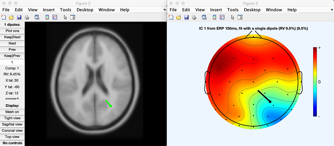
figure; pop_topoplot(TMPEEG,0,1, [ 'ERP 100ms, fit with a single dipole (RV ' num2str(dipole(1).rv*100,2) '%)'], 0, 1);

クリック詳しくはこちら上記のスクリプトをダウンロードします。スクリプトを実行すると、以下の2つのプロットが作成されます。

こちら

eLoretaソースローカリゼーションのためのシンプルなプラグインも利用可能です。このプラグインはミニマルなファッションで設計されており、他のプラグインのテンプレートとして使用できます。そのグラフィカルな出力は、次のセクションに示すスクリプトと同じです。

DIPFIT/FieldTrip ソース再構築

DIPFITは現在、FieldTripのソースイメージング機能を統合しています。Robert Oostenveldらがソースローカリゼーション機能をFieldTripとして開発し、DIPFITと統合されました。これにより、FieldTripの高度なソース解析機能をEEGLABのデータセットに直接適用できます。

まず、DIPFITでヘッドモデルを設定し、電極位置を共同登録します（メニュー項目ツール → DIPFIT → ヘッドモデルと設定）。DIPFIT 情報は、ソースのローカリゼーションを実行するために使用することができる FieldTrip

ボリュームでソースの再構築を実行

3D のフィールドライングリッド(eLoreta )

%% First load a dataset in EEGLAB.
% Then use EEGLAB menu item <em>Tools > Locate dipoles using DIPFIT > Head model and settings</em>
% to align electrode locations to a head model of choice
% The eeglab/fieldtrip code is shown below:

eeglab                        % start eeglab
eeglabPath = fileparts(which('eeglab'));                 % save its location
bemPath = fullfile(eeglabPath, 'plugins', 'dipfit', 'standard_BEM');    % load the dipfit plugin
EEG = pop_loadset(fullfile(eeglabPath, 'sample_data', 'eeglab_data_epochs_ica.set'));   % load the sample eeglab epoched dataset
EEG = pop_dipfit_settings( EEG, 'hdmfile',fullfile(bemPath, 'standard_vol.mat'), ...
           'coordformat','MNI','mrifile',fullfile(bemPath, 'standard_mri.mat'), ...
           'chanfile',fullfile(bemPath, 'elec', 'standard_1005.elc'), ...
           'coord_transform',[0.83215 -15.6287 2.4114 0.081214 0.00093739 -1.5732 1.1742 1.0601 1.1485] , ...
           'chansel',[1:32] );

次に、リードフィールド行列を ft_prepare_leadfield で計算します。ヘッドモデルも非常に注意与えられたボクセルが脳内外にあるかどうかを評価します。

%% Leadfield Matrix calculation
dataPre = eeglab2fieldtrip(EEG, 'preprocessing', 'dipfit');   % convert the EEG data structure to fieldtrip

cfg = [];
cfg.channel = {'all', '-EOG1'};
cfg.reref = 'yes';
cfg.refchannel = {'all', '-EOG1'};
dataPre = ft_preprocessing(cfg, dataPre);

vol = load('-mat', EEG.dipfit.hdmfile);

cfg            = [];
cfg.elec       = dataPre.elec;
cfg.headmodel  = vol.vol;
cfg.resolution = 10;   % use a 3-D grid with a 1 cm resolution
cfg.unit       = 'mm';
cfg.channel    = { 'all' };
[sourcemodel] = ft_prepare_leadfield(cfg);

次に、生成されたリードフィールド行列を使用してソース再構築を実行します。以下では、eLoreta を使用したシンプルな例を示します。このセクションは、FieldTrip のビームフォーマーチュートリアルを参照しています。

%% Compute an ERP in FieldTrip. Note that the covariance matrix needs to be calculated here for use in source estimation.
cfg                  = [];
cfg.covariance       = 'yes';
cfg.covariancewindow = [EEG.xmin 0]; % calculate the average of the covariance matrices
                                   % for each trial (but using the pre-event baseline  data only)
dataAvg = ft_timelockanalysis(cfg, dataPre);

% source reconstruction
cfg             = [];
cfg.method      = 'eloreta';
cfg.sourcemodel = sourcemodel;
cfg.headmodel   = vol.vol;
source          = ft_sourceanalysis(cfg, dataAvg);  % compute the source model

注意: ソリューションは低解像度のヘッドボリュームで生成されます。技術的には高解像度MRIに補間することも可能ですが、計算リソースが大きく必要になります（低解像度のヘッドモデルでもリードフィールド行列は既にかなり大きいため、高解像度への変換は非現実的です）。異なるボクセルやレイテンシーを選択して結果を確認してください。

また、プロットされたボリュームに不連続が見られる場合があります。これは、隣接するボクセル間でダイポールの方向の極性が突然反転するためです。空間と時間において、一時的な活動は継続的です。それでも、各ボクセルの3Dダイポールの方向は独立しており、隣接するボクセルは、反対の極性を持っているかもしれません(そして、のコース、反対に署名された時間コースも。理想的なソリューションは、スペースと時間の両方で反転を避けるためにまだ発見されていない - 持っているすべてのダイポールは、ヘッドセンターに敬意を表しています。関連するソース時間コースをそれに応じて反転 - は試してみる価値のあるソリューション。または、ダイポールの方向の異なる軸をプロットすることができます。

%% Plot Loreta solution
cfg = [];
cfg.projectmom = 'yes';
cfg.flipori = 'yes';
sourceProj = ft_sourcedescriptives(cfg, source);

cfg = [];
cfg.parameter = 'mom';
cfg.operation = 'abs';
sourceProj = ft_math(cfg, sourceProj);

cfg              = [];
cfg.method       = 'ortho';
cfg.funparameter = 'mom';
figure; ft_sourceplot(cfg, sourceProj);

![ボーダー

500px](/assets/images/Dipfiteloreta3.png)

興味の遅延が選択されたら、それらはにプロジェクトされるかもしれません高分解能MRIの強みテンプレートの脳のスライス。

%% project sources on MRI and plot solution
mri = load('-mat', EEG.dipfit.mrifile);
mri = ft_volumereslice([], mri.mri);

cfg              = [];
cfg.downsample   = 2;
cfg.parameter    = 'pow';
source.oridimord = 'pos';
source.momdimord = 'pos';
sourceInt  = ft_sourceinterpolate(cfg, source , mri);

cfg              = [];
cfg.method       = 'slice';
cfg.funparameter = 'pow';
ft_sourceplot(cfg, sourceInt);

![ボーダー

500px](/assets/images/Dipfiteloreta4.png)

表面にソースを再構築する

あるいは、下のコードは皮質表面上のリードフィールド行列を生成します。DIPFITのヘッドモデル設定で指定した座標系を使用します。異なるメッシュ解像度のバージョンが利用可能です。詳しくはこのFieldTripチュートリアルのための詳細情報。以下のコードは実行していると仮定します上記のコード。

%% Prepare leadfield surface
[ftVer, ftPath] = ft_version;
sourcemodel = ft_read_headshape(fullfile(ftPath, 'template', 'sourcemodel', 'cortex_8196.surf.gii'));

cfg           = [];
cfg.grid      = sourcemodel;    % source points
cfg.headmodel = vol.vol;        % volume conduction model
leadfield = ft_prepare_leadfield(cfg, dataAvg);

eLoretaの代わりに、最小ノルム推定（MNE）を使用することもできます。MNEおよびeLoretaのソース再構築は、各レイテンシーに対して実行され、時系列データを入力として使用します。

%% Surface source analysis
cfg               = [];
cfg.method        = 'mne';
cfg.grid          = leadfield;
cfg.headmodel     = vol.vol;
cfg.mne.lambda    = 3;
cfg.mne.scalesourcecov = 'yes';
source            = ft_sourceanalysis(cfg, dataAvg);

次に、グローバルパワーをプロットします。MNEソリューションの詳細については、FieldTripのチュートリアルページを参照してください。

%% Surface source plot
cfg = [];
cfg.funparameter = 'pow';
cfg.maskparameter = 'pow';
cfg.method = 'surface';
cfg.latency = 0.4;
cfg.opacitylim = [0 200];
ft_sourceplot(cfg, source);

![ボーダー

500px](/assets/images/FieldTrip_surface_solution2.png)

ソースモデルのメッシュのアライメントを視覚的に確認することもできます。 BEMヘッドモデルと重ね合わせて確認できます（下記参照）。

hold on; ft_plot_mesh(vol.vol.bnd(3), 'facecolor', 'red', 'facealpha', 0.05, 'edgecolor', 'none');
hold on; ft_plot_mesh(vol.vol.bnd(2), 'facecolor', 'red', 'facealpha', 0.05, 'edgecolor', 'none');
hold on; ft_plot_mesh(vol.vol.bnd(1), 'facecolor', 'red', 'facealpha', 0.05, 'edgecolor', 'none');

![ボーダー

500px](/assets/images/FieldTrip_surface_solution_with_bem2.png)

クリック詳しくはこちら上記のスクリプトをダウンロードします。

FieldTripチュートリアル

ソースを作成する方法モデルと利用可能なテンプレートソースモデル ( 1 つ上記で使用しているもの)
ボリューム伝導を定義する方法モデル
ビームフォーマーメソッド - 上記の例では ‘eloreta’ を ‘dics’ に置き換えて使用できます
最小限の規範見積り MEGの例ですが、EEGにも適用可能です
DIPFITのチュートリアル

このチュートリアルは Arnaud Delorme が作成し、Robert Oostenveld と Scott Makeig の協力を得ています。